Observer Horizon Profile

This notebook illustrates how to compute and visualise the real visible horizon as seen from any observing site, using the Observer.horizon_profile() method introduced in MontuPython.

The computation uses the Copernicus GLO-30 Digital Elevation Model (30 m / pixel, equivalent resolution to SRTM), downloaded automatically from the public AWS S3 bucket — no login or API key required.

Key features:

🌍 Automatic tile download and local caching (tiles are reused on repeated calls).
⚡ Fast two-phase radial scan: coarse grid + fine refinement around peaks.
🔭 Full Earth-curvature correction in the elevation-angle formula.
📈 Interactive Plotly chart of the horizon silhouette.
📐 Smooth get_elevation(azimuth) interpolation via scipy.

If you are running this notebook in Google Colab, install the required packages first:

[1]:

try:
    from google.colab import drive
    %pip install -Uq montu
except ImportError:
    print("Not running in Colab, skipping installation")
    import plotly.io as pio
    pio.renderers.default = "notebook_connected"
    %load_ext autoreload
    %autoreload 2
# Create folders for figures and temporal files
!mkdir -p ./gallery/ ./montu_dem/

Not running in Colab, skipping installation

[2]:

%matplotlib inline
import montu as mn

MontuPython version 0.50.0. 𓇍𓇋𓇋𓏏𓅓𓊵 𓎛𓎡𓄿𓀭𓎛𓈖𓂝𓎡 (ii-ti m Htp, HkAx Hn'-k)

The Horizon Class

In the base of the horizon calculation reside the Horizon class that can be instantiated with the information about the site:

[3]:

# Funerary temple of Senenmut, Luxor, Egypt
senenmut = mn.Horizon(
    lat=25.738258, lon=32.608913, alt_m=140.0,
    site_name='Funerary Temple of Senenmut'
)

senenmut.get_profile(max_dist=40, az_step=0.5, coarse_step=0.1)
print(senenmut)

Obtaining horizon profile...
Downloading DEMs (digital elevation maps) for this site. This can take a few seconds. Please be patient.
Horizon for 'Funerary Temple of Senenmut'
  Coordinates: lat=25.7383, lon=32.6089, alt=140 m
  Status: computed (720 pts)
  Elevation range: [0.02°, 21.21°]
  Parameters: max_dist=40 km, az_step=0.5°, coarse_step=0.1 km

The process of calculating the horizon profile involves:

Downloading the Copernicus GLO-30 TIFF tiles for the specified region.
Calculating the line of sight for each azimuth up to the maximum distance (max_dist).
Determining the maximum elevation angle while accounting for the Earth’s curvature.

Once you have calculated the horizon profile, you can use it for multiple purposes. The most simple one is generating an interactive plot of the horizon silhouette:

[4]:

fig = senenmut.plot_horizon()

As you can see, the default option plots the entire 360° horizon. You can also restrict your view to a particular direction and narrow the field of view (the parameters below represent a natural field of view for naked-eye observations):

[5]:

fig = senenmut.plot_horizon(az_center=221, az_delta=40, elev_view=30)

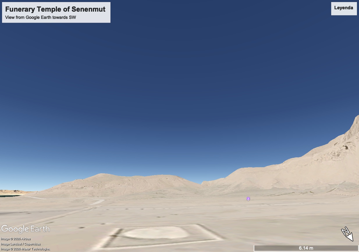
We can compare it to the Horizon shown by Google Earth:

By integrating MontuPython’s astronomical functionalities, we can overlay the sky onto the horizon at a specific date and time, accurately occluding stars behind local mountains:

[6]:

mtime = mn.Time('bce1460-01-01 20:00:00')
# Show the sky in a 180° window centred towards North (az=0)
fig = senenmut.plot_horizon(
    at=mtime,
    mag_limit=5,
    az_center=0,
    az_delta=90,
    elev_view=30, # optional: adjust elevation limit
    show_planets='all'
)

Loading stellar catalogue montu_stellar_catalogue_v38_visible.csv

Or including the Galaxy (blue thin and dashed lines):

[7]:

mtime = mn.Time('bce1460-01-01 09:30:00')
# Show the sky in a 180° window centred towards North (az=0)
fig = senenmut.plot_horizon(
    at=mtime,
    mag_limit=5,
    az_center=180,
    az_delta=90,
    elev_view=30, # optional: adjust elevation limit
    show_planets='all',
    show_constellation_lines=True,
    show_galaxy_equator=True,
    show_galaxy_contours=True,
)

An observer with horizon

An Observer is defined by its geodetic coordinates. The height parameter is in kilometres. Here we use the Universidad de Antioquia (Medellín, Colombia) as our first example site.

[8]:

mars = mn.Planet("Mars")
aldebaran = mn.Stars(subset="bright", ProperName="Aldebaran", return_as="Star")
site = mn.Observer(site="athens")
conj = mn.Conjunction(
    bodies=[mars, aldebaran],
    maxseparation=5,
    mtime=mn.Time("2022-09-07"),
    observer=site,
)
conj.show_details()
conj.plot_map()

Conjunction: Mars–Aldebaran
  Epoch (UTC)          : 2022-09-07 00:00:00
  Julian Day (UTC)     : 2459829.500000
  Observer             : lat 37.983800°, lon 23.727500°
  Local solar time     : 01:34:54.600
  Angular separation   : 4.2806° (max allowed 5.0°)
  In conjunction       : yes
  Sun altitude         : -40.47°
  Is visible from site : yes (bodies above horizon and Sun < -5°)
  Pair Mars–Aldebaran
    Separation         : 4.2806°
    Position angle     : 166.05° (N→E)
  Mars
    Elevation / azimuth: 37.14° / 91.62° (above horizon: yes)
    Rise (UTC)         : 2022-09-07 20:40:40
    Set (UTC)          : 2022-09-07 11:04:04
    Phase              : 85.39%
    Angular size       : 0.169 arcmin
    V magnitude        : -0.22
  Aldebaran
    Elevation / azimuth: 33.98° / 95.16° (above horizon: yes)
    Rise (UTC)         : 2022-09-07 20:57:57
    Set (UTC)          : 2022-09-07 10:52:52
    V magnitude        : 0.87

[9]:

# Universidad de Antioquia, Medellín, Colombia
udea = mn.Observer(lat=6.266152, lon=-75.569335, height=1.468)
print(udea)

Observer
  Coordinates: lat 6.266152°, lon -75.569335°, elevation 1468 m (1.468 km)
  Atmosphere: P=1013.25 mbar, T=15.0 °C, RH=0, λ=0.6 μm

Call Observer.horizon_profile() to:

Download the Copernicus DEM tiles that cover the area (skipped if already cached).
Run the two-phase radial scan (coarse + fine).
Store the result as observer.horizon (a montu.Horizon object).

Parameters:

Parameter	Default	Description
`max_dist`	30 km	Maximum search radius
`az_step`	1°	Azimuth resolution
`coarse_step`	3 km	Coarse scan spacing
`tmpdir`	`./montu_dem`	Cache directory for tiles

[10]:

udea.horizon_profile(
    max_dist=30,       # km
    az_step=1,         # degrees
    coarse_step=3,     # km
)
print(udea.horizon)

Obtaining horizon profile...
Downloading DEMs (digital elevation maps) for this site. This can take a few seconds. Please be patient.
Horizon for 'MontuSite (lat. 6.266152, lon. -75.569335, alt. 1468.0)'
  Coordinates: lat=6.2662, lon=-75.5693, alt=1468 m
  Status: computed (360 pts)
  Elevation range: [1.08°, 12.50°]
  Parameters: max_dist=30 km, az_step=1°, coarse_step=3 km

The information about the horizon is stored in:

[11]:

udea.horizon.data

[11]:

	azimuth	elevation	lat	lon	distance
0	0	4.423749	6.392057	-75.569335	14
1	1	4.589127	6.401030	-75.566966	15
2	2	4.921972	6.400968	-75.564598	15
3	3	5.004847	6.391884	-75.562704	14
4	4	5.538193	6.382779	-75.561129	13
...	...	...	...	...	...
355	355	3.891672	6.391578	-75.580377	14
356	356	3.979499	6.391750	-75.578173	14
357	357	4.061773	6.391884	-75.575966	14
358	358	4.404990	6.391980	-75.573757	14
359	359	4.514360	6.392038	-75.571546	14

360 rows × 5 columns

Querying the Horizon Elevation

After computing the profile, get_elevation(azimuth) returns the interpolated horizon elevation angle (in degrees) for any azimuth direction.

Convention: Azimuth is measured from North (0°) clockwise to East (90°), South (180°) and West (270°).

[12]:

directions = {'N': 0, 'NE': 45, 'E': 90, 'SE': 135, 'S': 180, 'SW': 225, 'W': 270, 'NW': 315}
for name, az in directions.items():
    elev = udea.horizon.get_elevation(az)
    print(f"Elevation looking {name:2s} ({az:3d}°): {elev:5.2f}°")

Elevation looking N  (  0°):  4.42°
Elevation looking NE ( 45°):  5.68°
Elevation looking E  ( 90°): 11.99°
Elevation looking SE (135°):  7.63°
Elevation looking S  (180°):  4.26°
Elevation looking SW (225°):  3.97°
Elevation looking W  (270°):  5.42°
Elevation looking NW (315°):  9.55°

Plotting the Horizon

plot_horizon() generates an interactive Plotly chart of the full 360° horizon silhouette. The dashed line at 0° marks the geometric (flat-earth) horizon.

[13]:

fig = udea.horizon.plot_horizon(az_center=0, elev_view=15)

You can also project the points forming the horizon onto a geographic 2D map to visualize the surrounding terrain:

[14]:

fig = udea.horizon.plot_map()

You can focus the map view on a specific direction. For example, in the plot below we restrict the azimuth range towards Robledo (a mountainous district in western Medellín):

WARNING: The map will not appear in browsers that do not support WebGL (such as in this static documentation).

[15]:

fig = udea.horizon.plot_horizon(az_center=315, az_delta=40, elev_view=15)

As shown earlier, you can dynamically plot the stars that are visible from this specific site at a given local time, taking the real horizon topography into account:

[16]:

mtime = mn.Time('2026-01-01 19:00:00', zone=udea)
# Show the sky in a 40° window centred towards North (az=0)
fig = udea.horizon.plot_horizon(
    at=mtime,
    mag_limit=5,
    az_center=0,
    az_delta=40,
    elev_view=30, # optional: adjust elevation limit
    show_constellation_lines=True,
    show_constellation_boundaries=True,
)

Using a Predefined Site

When an Observer is created from a predefined site in the MontuPython catalogue (e.g. site='thebes'), horizon_profile() automatically picks up the site name for the chart title.

[17]:

# Ancient Thebes (Luxor), Egypt
thebes = mn.Observer(site='thebes')
print(thebes)

Observer
  Site: Thebes (Luxor) [thebes]
  Region: Egypt · Ancient Egypt
  Coordinates: lat 25.696700°, lon 32.642200°, elevation 76 m (0.076 km)
  Atmosphere: P=1004.16 mbar, T=25.2 °C, RH=0, λ=0.6 μm
  Description: Ancient Waset — capital of Upper Egypt during the New Kingdom. Karnak and the Valley of the Kings lie nearby.

[18]:

thebes.horizon_profile(max_dist=30, az_step=1, coarse_step=3)
print(thebes.horizon)

Obtaining horizon profile...
Downloading DEMs (digital elevation maps) for this site. This can take a few seconds. Please be patient.
Horizon for 'Thebes (Luxor)'
  Coordinates: lat=25.6967, lon=32.6422, alt=76 m
  Status: computed (360 pts)
  Elevation range: [-0.02°, 3.24°]
  Parameters: max_dist=30 km, az_step=1°, coarse_step=3 km

[19]:

fig = thebes.horizon.plot_horizon(az_center=315, az_delta=30, elev_view=15)

These are the mountains on the West Bank of Thebes, in the general direction of the Valley of the Kings.

High-Resolution Profile

Decrease az_step and coarse_step to get a more detailed profile. Because the DEM is read locally (no network round-trips), even very dense grids complete in a few seconds.

[20]:

# Valley of the Kings, Luxor, Egypt
vok = mn.Observer(lat=25.739998, lon=32.600985, height=0.188)

vok.horizon_profile(
    max_dist=30,
    az_step=0.5,      # finer azimuth resolution
    coarse_step=0.1,    # finer coarse scan
)
print(vok.horizon)
vok.horizon.site_name = 'Valley of the Kings'
fig = vok.horizon.plot_horizon(az_center=225, az_delta=40)

Obtaining horizon profile...
Downloading DEMs (digital elevation maps) for this site. This can take a few seconds. Please be patient.
Horizon for 'MontuSite (lat. 25.739998, lon. 32.600985, alt. 188.0)'
  Coordinates: lat=25.7400, lon=32.6010, alt=188 m
  Status: computed (720 pts)
  Elevation range: [0.47°, 22.00°]
  Parameters: max_dist=30 km, az_step=0.5°, coarse_step=0.1 km

Here we can see the classical pyramid-shaped mountain of el-Qurn.

Working Directly with the Horizon Object

You can also instantiate montu.Horizon independently and call get_profile() on it, if you prefer not to go through Observer.

[21]:

# Funerary temple of Senenmut, Luxor, Egypt
senenmut = mn.Horizon(
    lat=25.738258, lon=32.608913, alt_m=140.0,
    site_name='Funerary Temple of Senenmut'
)

senenmut.get_profile(max_dist=40, az_step=1, coarse_step=0.1)
print(senenmut)

Obtaining horizon profile...
Horizon for 'Funerary Temple of Senenmut'
  Coordinates: lat=25.7383, lon=32.6089, alt=140 m
  Status: computed (360 pts)
  Elevation range: [0.02°, 21.21°]
  Parameters: max_dist=40 km, az_step=1°, coarse_step=0.1 km

[22]:

fig = senenmut.plot_horizon(az_center=221, az_delta=40, elev_view=None)

[23]:

fig = senenmut.plot_horizon(az_center=180, az_delta=180, elev_view=None)

[24]:

mtime = mn.Time('bce1460-01-01 20:00:00')
# Show the sky in a 90° window centred towards North (az=0)
fig = senenmut.plot_horizon(
    at=mtime,
    mag_limit=5,
    az_center=0,
    az_delta=90,
    elev_view=30 # optional: adjust elevation limit
)

Akhetaten

One of the most fascinating examples of the relationship between the horizon and the sky occurred in the ancient city of Akhetaten (modern Amarna):

[25]:

site = mn.Observer(site='amarna')
site.horizon_profile(
    max_dist=30,       # km
    az_step=.5,         # degrees
    coarse_step=0.1
)

Obtaining horizon profile...

[25]:

Horizon: lat=27.6444, lon=30.9014, alt=90 m, computed, 720 pts, elev [-0.22°, 1.22°]

Let’s calculate and visualize the entire 360° horizon profile for the site:

[26]:

fig = site.horizon.plot_horizon()

Let’s focus the plot on the Royal Wadi, located towards the east:

[27]:

fig = site.horizon.plot_horizon(az_center=90, az_delta=40, elev_view=5)

That distinctive ‘dip’ or wadi at azimuth 103° held profound religious significance for the ancient Egyptians. Let’s compute and plot the sunrise during the time of Akhenaten to see why:

Sun rising in the Akhet-aten

First, we calculate the local time of sunrise near the foundation date of the city:

[28]:

sun = mn.Sun()
mtime_initial = mn.Time('bce1341-10-21')
sun.conditions_in_sky(at=mtime_initial, observer=site)
jd_sun_rise = sun.condition.rise_time
mtime_rise = mn.Time(sun.condition.rise_time, format='jd')
site.get_local_time(sun.condition.rise_time), mtime_rise, sun.condition.rise_az

[28]:

('06:10:12.448',
 Time('-1340-10-21 04:06:36.103664'/'-1340-11-02 04:06:06'/'[hrw 1442] IV akhet 12'/JED 1231928.6712512/JTD 1231929.0408565),
 102.30066093548338)

[29]:

fig = site.horizon.plot_horizon(
    at=mtime_rise,
    mag_limit=5,
    az_center=90,
    az_delta=40,
    elev_view=2, # adjust to see the Sun emerge
    show_constellation_lines=False,
)

As you can see at the time of rising as computed by the library, the sun is even below the horizon. This is because, by the default at the atmospheric pressure of the observer, the atmospheric refraction is around 0.5 degrees. On the other hand the library computes the elevation with respect to the mathematical or geometrical horizon.

MontuPython allows to refine the conditions of rise and setting including the horizon of the observer:

[30]:

sun = mn.Sun()
mtime_initial = mn.Time('bce1341-10-21')
sun.conditions_in_sky(at=mtime_initial, observer=site, horizon=True)

mtime_rise_hor = mn.Time(sun.condition.rise_time_hor, format='jd')
site.get_local_time(sun.condition.rise_time_hor), mtime_rise, sun.condition.rise_az_hor

[30]:

('06:15:42.721',
 Time('-1340-10-21 04:06:36.103664'/'-1340-11-02 04:06:06'/'[hrw 1442] IV akhet 12'/JED 1231928.6712512/JTD 1231929.0408565),
 102.9391880002312)

[31]:

sun.condition.set_az, sun.condition.set_az_hor, sun.condition.rise_az, sun.condition.rise_az_hor

[31]:

(257.50274891735967, 257.3150826397244, 102.30066093548338, 102.9391880002312)

[32]:

fig = site.horizon.plot_horizon(
    at=mtime_rise_hor,
    az_center=90,
    az_delta=40,
    elev_view=4,
    mag_limit=0,
    show_constellation_lines=False,
    show_star_names=False,
    show_planets=['Sun', 'Moon']
)

[33]:

fig = site.horizon.plot_horizon(
    at=mtime_rise_hor,
    az_center=90,
    az_delta=40,
    elev_view=4,
    mag_limit=-1,
    show_constellation_lines=False,
    show_star_names=False,
    show_planets=['Sun']
)

The stars of the North shaft of the Khufu great pyramid

The Great Pyramid of Giza features enigmatic ‘air shafts’ pointing towards specific regions of the sky. The northern shaft of the King’s Chamber has an inclination of approximately 31.4°, seemingly aligned towards the circumpolar stars of the Pyramid age (around 2550 BCE). Let us use MontuPython to investigate the sky and horizon at Giza and verify this famous alignment.

[34]:

site = mn.Observer(site='giza')
site.horizon_profile(
    max_dist=30,       # km
    az_step=0.5,         # degrees
    coarse_step=0.1,     # km
)

Obtaining horizon profile...
Downloading DEMs (digital elevation maps) for this site. This can take a few seconds. Please be patient.

[34]:

Horizon: lat=29.9792, lon=31.1342, alt=75 m, computed, 720 pts, elev [-0.24°, 2.85°]

It is traditionally believed that Thuban was the star targeted by the north shaft. Let us compute the culmination (transit) time of this star:

[35]:

star = mn.Stars(ProperName='Thuban', return_as='Star')
mtime = mn.Time('bce2550-01-01 00:00:00', zone=site)
star.conditions_in_sky(at=mtime, observer=site)
mtime_transit = mn.Time(star.condition.transit_time, format='jd')

Loading stellar catalogue montu_stellar_catalogue_v38.csv

Now let us look at the horizon at that time:

[36]:

fig = site.horizon.plot_horizon(
    at=mtime_transit,
    az_center=0,
    az_delta=40,
    elev_view=45,
    mag_limit=6,
    show_constellation_lines=True,
    show_star_names=True,
    show_planets=None,
    show_constellation_labels=True,
    #constellation_set='egyptian_ancient', #Other: 'egyptian_dendera', by default: 'iau'
    #constellation_set='egyptian_dendera',
)

We can verify that the elevation of Thuban at transit is exactly 31.4°, matching the inclination of the shaft.

Can yo recognize the pyramids:

[37]:

fig = site.horizon.plot_horizon(
    az_center=90,
    az_delta=180,
    elev_view=5,
    show_title=False,
)

It is a good idea that after using Horizons, clean your caches of DEM files:

[38]:

# mn.Horizon.clean_cache(verbose=True)

Powered by MontuPython. For more examples see MontuPython GitHub repo.